Interactive, annotatable, code-driven presentations

Achintya Rao

19 May 2017

1 Bookdown example

1.1 The inspiration!

D3 visualisations by Eamonn Maguire

• Creating Visualizations with D3 by Eamonn Maguire

1.2 Using R code in your presentation

1.2.1 Example of some code

summary(mtcars)

##       mpg             cyl             disp             hp       
##  Min.   :10.40   Min.   :4.000   Min.   : 71.1   Min.   : 52.0  
##  1st Qu.:15.43   1st Qu.:4.000   1st Qu.:120.8   1st Qu.: 96.5  
##  Median :19.20   Median :6.000   Median :196.3   Median :123.0  
##  Mean   :20.09   Mean   :6.188   Mean   :230.7   Mean   :146.7  
##  3rd Qu.:22.80   3rd Qu.:8.000   3rd Qu.:326.0   3rd Qu.:180.0  
##  Max.   :33.90   Max.   :8.000   Max.   :472.0   Max.   :335.0  
##       drat             wt             qsec             vs        
##  Min.   :2.760   Min.   :1.513   Min.   :14.50   Min.   :0.0000  
##  1st Qu.:3.080   1st Qu.:2.581   1st Qu.:16.89   1st Qu.:0.0000  
##  Median :3.695   Median :3.325   Median :17.71   Median :0.0000  
##  Mean   :3.597   Mean   :3.217   Mean   :17.85   Mean   :0.4375  
##  3rd Qu.:3.920   3rd Qu.:3.610   3rd Qu.:18.90   3rd Qu.:1.0000  
##  Max.   :4.930   Max.   :5.424   Max.   :22.90   Max.   :1.0000  
##        am              gear            carb      
##  Min.   :0.0000   Min.   :3.000   Min.   :1.000  
##  1st Qu.:0.0000   1st Qu.:3.000   1st Qu.:2.000  
##  Median :0.0000   Median :4.000   Median :2.000  
##  Mean   :0.4062   Mean   :3.688   Mean   :2.812  
##  3rd Qu.:1.0000   3rd Qu.:4.000   3rd Qu.:4.000  
##  Max.   :1.0000   Max.   :5.000   Max.   :8.000

1.2.2 Inline code

So, sqrt(81)*4*pi becomes 113.0973355.

1.2.3 Import some data

I_jean <- read.delim("http://bit.ly/avml_ggplot2_data")
head(I_jean)

##    Name Age Sex Word FolSegTrans Dur_msec     F1     F2      F1.n
## 1 Jean   61   f  I'M           M      130  861.7 1335.8 1.6608625
## 2 Jean   61   f    I           N      140 1010.4 1349.3 2.6882695
## 3 Jean   61   f I'LL           L      110  670.1 1292.7 0.3370482
## 4 Jean   61   f  I'M           M      180  869.8 1307.0 1.7168275
## 5 Jean   61   f    I           R       80  743.0 1418.7 0.8407333
## 6 Jean   61   f I'VE           V      120  918.2 1580.8 2.0512357
##         F2.n
## 1 -0.8855366
## 2 -0.8536494
## 3 -0.9873394
## 4 -0.9535626
## 5 -0.6897257
## 6 -0.3068434

• Source: https://jofrhwld.github.io/avml2012/

1.2.4 Static plots

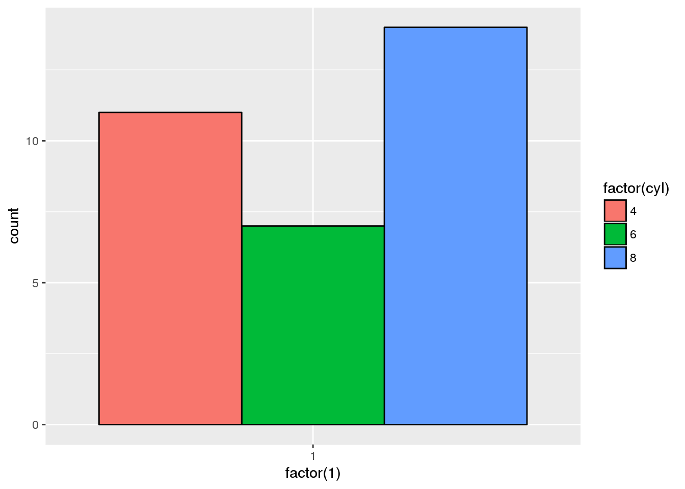
1.2.5 Interactive plots!

1.2.6 Make more plots!

1.3 Making a reveal.js presentation

1.3.1 R Markdown with embedded R code

• Source
• Hosted on GitHub: RaoOfPhysics/contained-revealr
• Displayed using GitHub Pages: raoofphysics.github.io/contained-revealr
• Annotatable using Hypothesis:
  • Add <script src="https://hypothes.is/embed.js" async></script>

1.3.2 The source file itself

• Create a new R Markdown file named index.Rmd
  • Select reveal.js from templates
• Add YAML frontmatter!
• Instructions for reveal.js presentations: rmarkdown.rstudio.com/revealjs_presentation_format.html
• Create sections and add content+code
• Knit your presentation!

1.4 “But I hate / don’t use R…”

1.4.1 Other “engines” for code chunks

Language	In RMarkdown	Plotly available
Python	Yes	Yes
JavaScript	Yes	Yes
SQL	Yes	No
Bash	Yes	No

More: http://rmarkdown.rstudio.com/authoring_knitr_engines.html

1.5 “But I don’t want to install R and its packages…”

1.5.1 RStudio via Docker

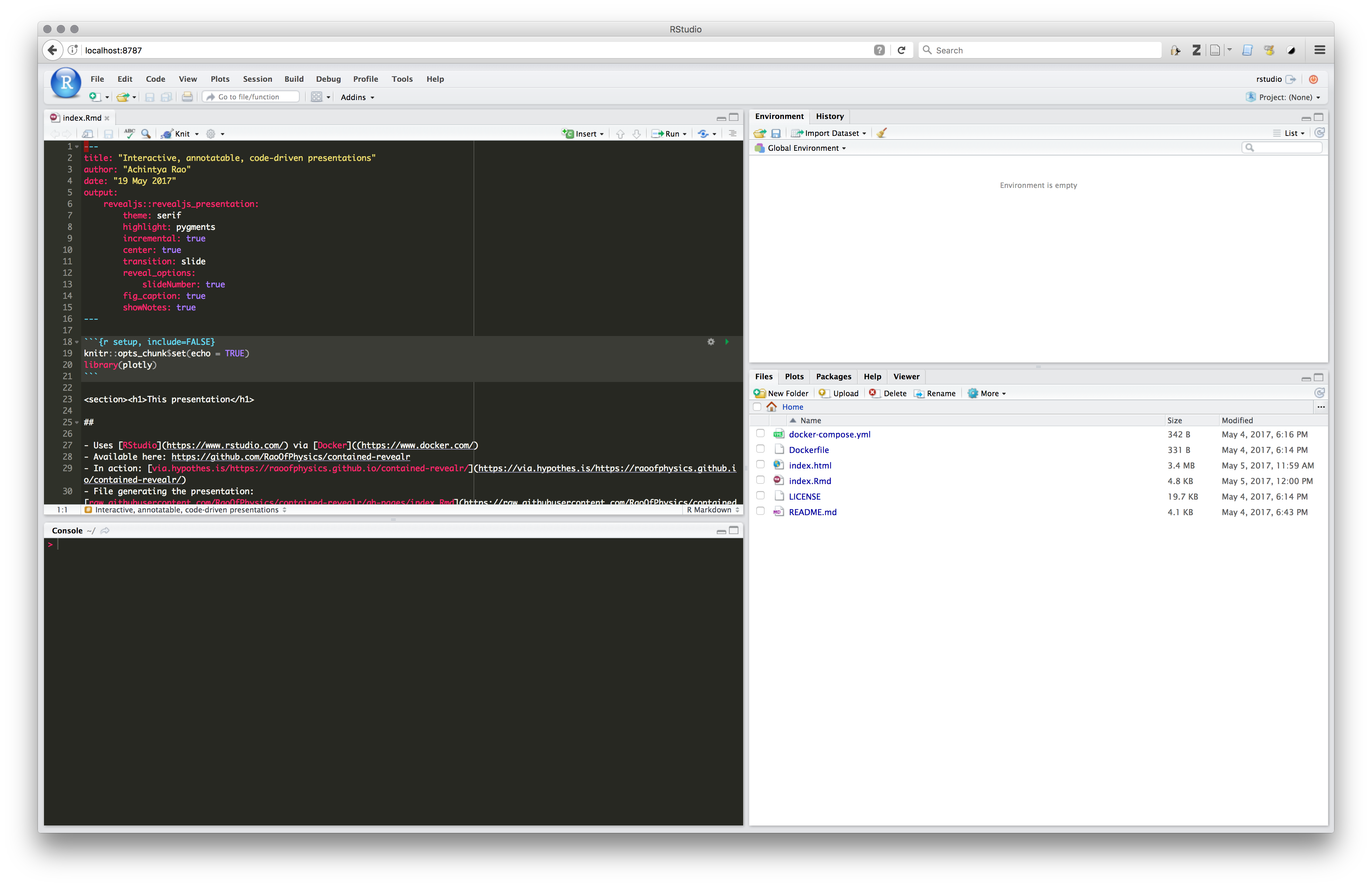
RStudio via Docker

1.5.2 Using RStudio in your browser

• Caveat! Non-R engines don’t work out of the box
• Create a directory for your project
• Add this Dockerfile and this docker-compose.yml to the directory
• Run $ docker-compose up -d
• Open RStudio in your browser at localhost:8787 or 0.0.0.0:8787
• Log in with “rstudio” as both the username and password
• To shutdown: $ docker-compose down

1.6 Questions?